Knowledge Graph
Visually explore the entities, relationships, and concepts extracted from your documents.
What is the Knowledge Graph?
Every RAG index automatically builds a Knowledge Graph alongside the vector index. While the vector index lets you ask questions in natural language, the knowledge graph gives you a visual map of what your documents contain - the people, organizations, concepts, events, and how they connect.
The graph is built automatically during indexing. You don't configure or maintain it - it grows and updates every time your index is rebuilt or updated.
How the Graph is Built
During indexing, after each document is chunked and embedded, an AI model reads the full document text and extracts:
- Entities - named things: people, organizations, locations, concepts, events, products, and more
- Relationships - directed connections between entities, with a description and a weight representing how strongly they are connected
Each entity is then scored by importance - a normalized 0–1 score computed from two factors:
| Factor | Weight |
|---|---|
| Mention count | How many text chunks across your documents contain this entity |
| Relationship count | How many connections this entity has in the graph (×2 weight) |
A score of 1.0 means the most central entity in your index. Scores close to 0 indicate peripheral mentions.
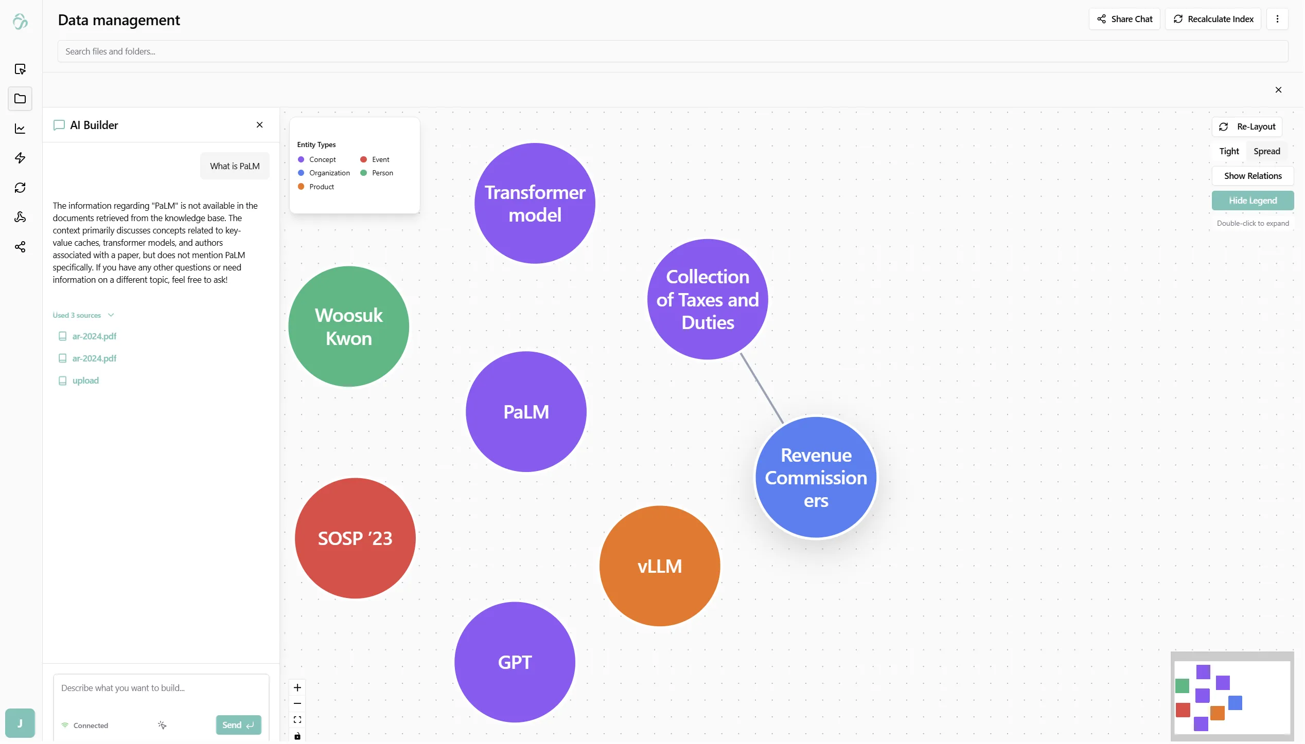
Graph Hierarchy
The knowledge graph uses a hierarchical navigation model - rather than loading all nodes at once (which becomes unusable at scale), you explore the graph level by level.
Level 1 - Cluster Centers
The initial view shows one representative node per cluster. The graph is partitioned into communities using the Louvain algorithm - a fast community detection method that groups densely connected entities together. The representative of each cluster is the most central node within that community.
This means:
- Every part of your data is always reachable from the first view
- No important cluster is buried or hidden
- The number of nodes shown equals the number of detected communities - typically between 5 and 30 for real document sets
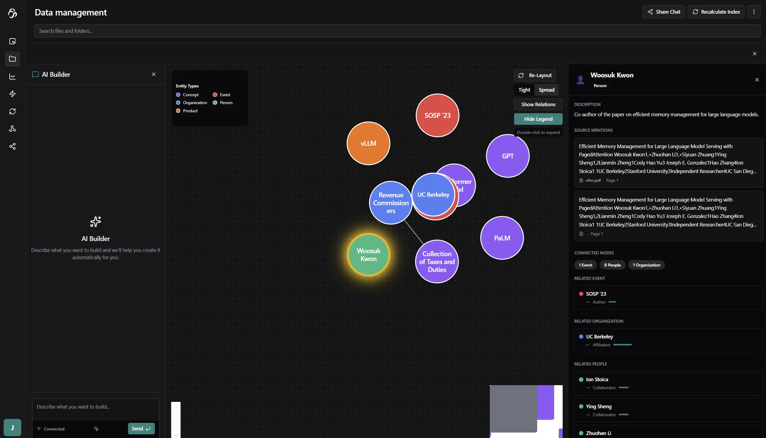
Level 2+ - Expanding a Node
Click any node to expand it. The view transitions to show that entity and all its direct neighbors - every entity it has a documented relationship with. Edges show the relationship type and direction; edge thickness reflects the accumulated connection weight.
You can keep clicking deeper into the graph from any node.
Full Graph
Use the Spread / Tight toggle and layout controls in the top right to adjust how the graph is displayed. To see all entities and relationships at once, this is available via the graph controls.
Entity Detail Panel
Click any node to open its detail panel on the right side of the graph.
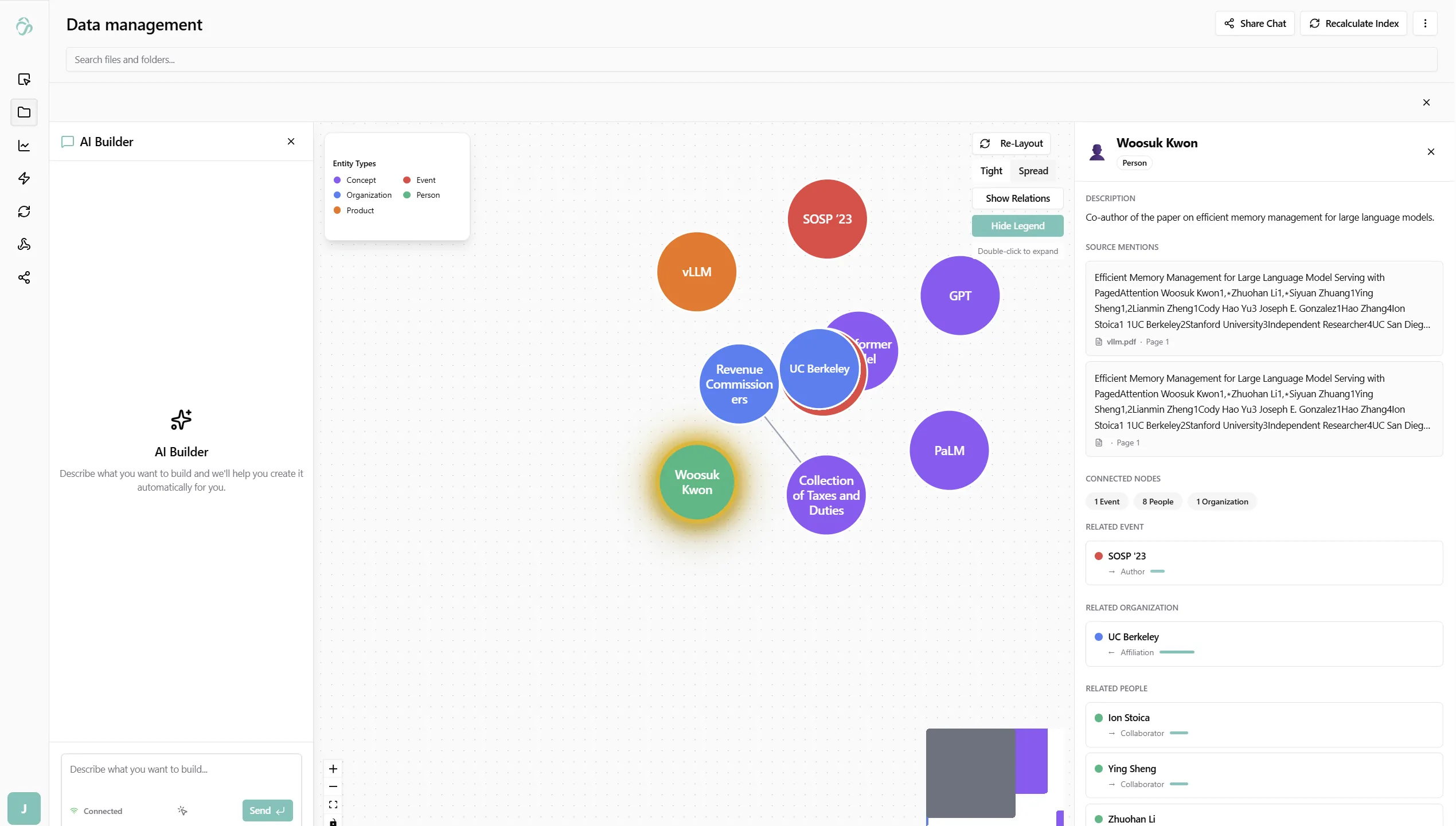
The panel shows:
- Name and type - the entity as extracted and classified by the AI
- Description - a short summary generated during extraction
- Source mentions - the document passages where this entity appears, with snippets
- Related events - events this entity is associated with
- Related organizations - organizations connected to this entity
- Related people - people connected to this entity
Each related item is clickable - clicking navigates to that entity's node in the graph.
Reading the Graph
Node size reflects the importance score - larger nodes are more central to your documents.
Edge thickness reflects the accumulated connection weight - thicker edges mean the relationship was found in more passages or was stated with greater emphasis. When multiple passages describe the same relationship, the weights are summed into a single edge rather than showing duplicate lines.
Edge direction shows the relationship direction - an arrow from A → B means A relates to B (e.g., "Woosuk Kwon co-authored with SOSP '23").
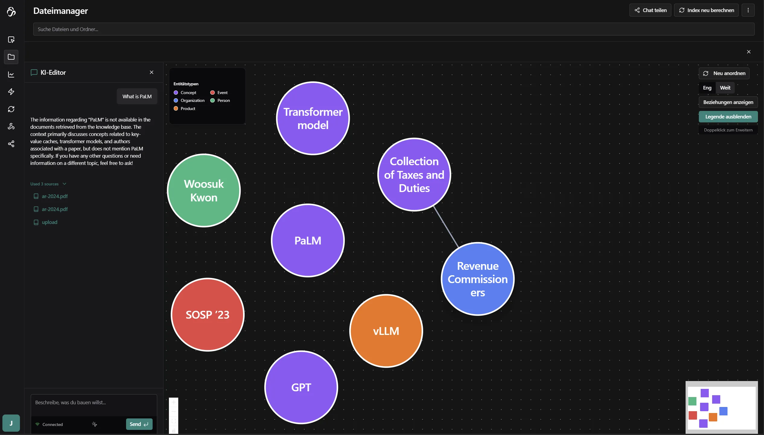
Node color groups entities by type - each entity type (person, organization, concept, event, product, etc.) gets a consistent color shown in the Entity Types legend.
Layout Controls
Use the controls in the top right of the graph to adjust the view:
| Control | Effect |
|---|---|
| Re-Layout | Re-runs the force-directed layout algorithm to untangle overlapping nodes |
| Tight / Spread | Adjusts how compressed or spread out the graph is |
| Show Relations | Toggles edge labels on/off |
Practical Uses
- Before querying - explore the graph to understand what entities your documents cover, so you can ask better questions
- Gap detection - if an entity you expect is absent or small, the relevant documents may not be indexed yet
- Relationship mapping - quickly see how two entities are connected across your documents without reading everything
- Topic clustering - clusters naturally correspond to sub-topics in your data (e.g., regulatory documents cluster separately from product specs)
- Source lookup - click a node and expand its source mentions to jump directly to the passages where it appears
Examples
Pharmaceutical R&D - Mapping a Clinical Program
A research team indexed 40 drug development reports spanning preclinical studies, Phase 1 and Phase 2 trials. After indexing, the graph clustered into four distinct communities: Compounds, Clinical Sites, Investigators, and Regulatory Bodies.
The compound node for their lead asset had the highest importance score (0.91) and was connected to 6 clinical sites, 18 investigators, and a direct edge to a regulatory submission filed by a CRO. That CRO relationship appeared in only two documents - but the graph surfaced it as a meaningful connection because both documents referenced it in proximity to safety data.
The team used the graph to orient themselves before opening the RAG chat - knowing the entity landscape meant they asked sharper questions and got more precise answers.
M&A Due Diligence - Spotting a Key Person Dependency
A deal team loaded a 200-document data room into a flow. After indexing, the graph's Key Personnel cluster immediately stood out: one node - a named technical co-founder - had unusually high relationship count, connected to 4 patent nodes, 2 subsidiary nodes, and a licensing agreement.
None of the executive summaries called this out explicitly. The graph surfaced it because the AI extracted the co-founder's name across documents that the deal team hadn't yet read. They clicked through to the source mentions and confirmed a key-person dependency that changed how they structured an earnout clause.
The same relationship map would have taken days to reconstruct manually from the raw documents.
Market Research - Validating a Hypothesis Before Reading
An analyst team indexed 30 sell-side research reports on the EV market to prepare a thematic summary. Before asking a single chat question, they opened the graph.
Battery supply chain was the highest-importance node (score 0.94), connected to 11 manufacturer nodes, 4 regulatory nodes, and 6 macroeconomic indicator nodes. The cluster structure confirmed their hypothesis - supply chain constraints were the dominant theme - and the edge labels showed how the reports were framing the issue: mostly as a cost risk, not a volume risk.
They went into the chat knowing exactly what to ask, which reduced the back-and-forth needed to get a useful synthesis.
Engineering - Tracing an Incident Pattern
An engineering team indexed three years of post-mortems, on-call runbooks, and architecture decision records. A recurring database stability issue had appeared in multiple incidents but was never formally linked.
In the graph, a PostgreSQL connection pool node had a high relationship count, connected to 4 separate incident nodes across different time periods. Clicking it revealed source mentions from three distinct post-mortems - each describing the same misconfiguration in slightly different language, which is why keyword search had never surfaced the pattern.
The team exported the cluster as context into the RAG chat and asked: "What is the common root cause across all connection pool incidents and what fixes were applied?" - getting a consolidated answer that synthesized all four post-mortems at once.
Responsible Developers: Julia, Usama, Aman.